MS Excel 2003 Training 202- Data Consolidation

To summarize and report results from multiple worksheets, you can consolidate data from each worksheet into a master worksheet. The worksheets can be in the same workbook or other workbooks. When you consolidate data, you are assembling data so you can more easily update and aggregate it on a regular or ad hoc basis.

For example, if you have a worksheet of expense figures for each of your regional offices, you might use a consolidation to roll up these figures into a corporate expense worksheet. This master worksheet might contain sales totals and averages, current inventory levels, and highest selling products for the entire enterprise.

To consolidate data, you use the Consolidate command from the Data menu to display the Consolidate dialog box. You can use this dialog box in several ways to consolidate your data:

Position  Use this approach when the data in all worksheets is arranged in identical order and location.
Category  Use this approach when each worksheet organizes the data differently, but has the same row and column labels, which you can use to match the data.
3-D formulas  Use this approach when the worksheets do not have a consistent pattern you can rely on. You can create formulas that refer to cells in each range of data that you're combining. Formulas that refer to cells on multiple worksheets are called 3-D formulas.

Consolidate by position

Consolidate by position when the data in all source areas is arranged in identical order and location; for example, if you have data from a series of worksheets that were created from the same template, you can consolidate the data by position.
You can set up the consolidation to update automatically when the source data changes, but you won't be able to change which cells and ranges are included in the consolidation. Or you can update the consolidation manually, allowing you to change the included cells and ranges.

Consolidate by category

Consolidate by category when you want to summarize a set of worksheets that have the same row and column labels but organize the data differently. This method combines data that has matching labels from each worksheet.
You can set up the consolidation to update automatically when the source data changes, but you won't be able to change which cells and ranges are included in the consolidation. Alternatively, you can update the consolidation manually, allowing you to change the included cells and ranges.

Consolidate by using 3-D formulas

When you use 3-D references (3-D reference: A reference to a range that spans two or more worksheets in a workbook.) in formulas, there are no restrictions on the layout of the separate ranges of data. You can change the consolidation any way you need to. The consolidation updates automatically when the data in the source ranges changes.
Use formulas to combine data   In the following example, the formula in cell A2 adds three numbers that are located in different positions on three different worksheets.



Add data to a consolidation with 3-D references   When all of your source worksheets have the same layout, you can use a range of sheet names in 3-D formulas. To add another worksheet to the consolidation, just move the sheet into the range your formula refers to.



Other ways to combine data

You can create a PivotTable report

MS Excel 2003 Training 101 - SUMIF and COUNTIF

SUMIF

Adds the cells specified by a given criteria.
Syntax
SUMIF(range,criteria,sum_range)

Range   is the range of cells that you want evaluated by criteria.
Criteria   is the criteria in the form of a number, expression, or text that defines which cells will be added. For example, criteria can be expressed as 32, "32", ">32", or "apples".
Sum_range   are the actual cells to add if their corresponding cells in range match criteria. If sum_range is omitted, the cells in range are both evaluated by criteria and added if they match criteria.
Remarks
Sum_range does not have to be the same size and shape as range. The actual cells that are added are determined by using the top, left cell in sum_range as the beginning cell, and then including cells that correspond in size and shape to range. For example:



You can use the wildcard characters, question mark (?) and asterisk (*), in criteria. A question mark matches any single character; an asterisk matches any sequence of characters. If you want to find an actual question mark or asterisk, type a tilde (~) preceding the character.
Microsoft Office Excel provides additional functions that you can use to analyze your data based on a condition or criteria:

To count the number of occurrences of a string of text or a number within a range of cells, use the COUNTIF function.
To have a formula return one of two values based on a condition, such as a sales bonus based on a specified sales amount, use the IF function.
To analyze data in a list based on criteria, such as profit margins or product types, use the database and list management functions (DAVERAGE, DCOUNT, DCOUNTA, DGET, DMAX, DMIN, DPRODUCT, DSTDEV, DSTDEVP, DSUM, DVAR, and DVARP).



COUNTIF

Counts the number of cells within a range that meet the given criteria.
Syntax
COUNTIF(range,criteria)

Range  is the range of cells from which you want to count cells.
Criteria  is the criteria in the form of a number, expression, cell reference, or text that defines which cells will be counted. For example, criteria can be expressed as 32, "32", ">32", "apples", or B4.
Remarks
You can use the wildcard characters, question mark (?) and asterisk (*), in criteria. A question mark matches any single character; an asterisk matches any sequence of characters. If you want to find an actual question mark or asterisk, type a tilde (~) before the character.
Microsoft Excel provides additional functions that can be used to analyze your data based on a condition.
To calculate a sum based on a string of text or a number within a range, use the SUMIF worksheet function.
To have a formula return one of two values based on a condition, such as a sales bonus based on a specified sales amount, use the IF worksheet function.
To count cells that are empty or not empty, use the COUNTA and COUNTBLANK functions.

Example 1: Common COUNTIF formulas



Example 2: COUNTIF formulas using wildcard characters and handling blank values



Note To view the number as a percentage, select the cell and click Cells on the Format menu. Click the Number tab, and then click Percentage in the Category box.

MS Excel 2003 Training 101 - Conditional Formulas

Testing whether conditions are true or false and making logical comparisons between expressions are common to many tasks. You can use the AND, OR, NOT, and IF function to create conditional formulas.
The IF function uses the following arguments.



Formula with the IF function

 logical_test: The condition that you want to check.
 value_if_true: The value to return if the condition is true.
 value_if_false: The value to return if the condition is false.

What do you want to do?
Create a conditional formula that results in a logical value (TRUE or FALSE)
Create a conditional formula that results in another calculation or in values other than TRUE or FALSE
Create a conditional formula that results in a logical value (TRUE or FALSE)
To do this task, use the AND, OR, and NOT functions, and operators (operator: A sign or symbol that specifies the type of calculation to perform within an expression. There are mathematical, comparison, logical, and reference operators.).



Create a conditional formula that results in another calculation or in values other than TRUE or FALSE

To do this task, use the IF, AND, and OR functions.



Advanced If statement usage:
Using multiple criteria with the “AND” and “OR” functions

Sometimes you need to check more than one criteria with the If statement. For example:
Only if the student has grades greater than 80 in Math, greater than 80 in English and greater than 80 in History, only then write “good student”, else write “Average Student”.


The way to implement such a case is using the “AND” function which will include all the multiple criteria inside of it.
This “AND” function, is then put inside the criteria section of the If statement.
Thus for the above example, the whole function could look something like this:


=IF(AND(C1>80,D1>80,E1>80) , “Good student” , “Average Student” )

Note that the criteria part: AND(C1>80,D1>80,E1>80) will be met only if all three parts of it are met.


The function “OR” is used in a same manner, but its meaning is slightly different.
Instead of checking if all its parts is met (as is the case of the “AND” function), it checks if at least one of the criteria inside it is met. If it is, then the whole “OR” is considered met.


Hence, in the following formula:

=IF(OR(C1>80,D1>80,E1>80) , “Good student” , “Average Student” )

It is enough that C1 is really greater than 80 , or that D1 is really greater than 80 or that E1 is really greater than 80 (or some combination of these three), to have the if function write “Good student”. Only if none of these cells (C1, D1 or E1) are greater than 80 the If function will result writing “Average Student”.

MS Excel 2003 Training 101 - Group and Outline

If you have a list of data that you want to group and summarize, you can create an outline of up to eight levels, one for each group. Each inner level, represented by a higher number in the outline symbols (outline symbols: Symbols that you use to change the view of an outlined worksheet. You can show or hide detailed data by pressing the plus sign, minus sign, and the numbers 1, 2, 3, or 4, indicating the outline level.) displays detail data (detail data: For automatic subtotals and worksheet outlines, the subtotal rows or columns that are totaled by summary data. Detail data is typically adjacent to and either above or to the left of the summary data.) for the preceding outer level, represented by a lower number in the outline symbols. Use an outline to quickly display summary rows or columns, or to reveal the detail data for each group.

You can create an outline of rows (as shown in the example to the left), an outline of columns, or an outline of both rows and columns.
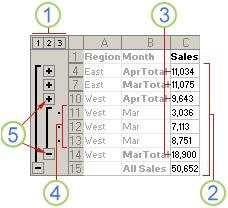
An outlined row of sales data grouped by geographical regions and months with several summary and detail rows displayed.


   To display rows for a level, click the appropriate outline symbols.
  Level 1 contains the total sales for all detail rows.
  Level 2 contains total sales for each month in each region.
  Level 3 contains detail rows (only detail rows 11 through 13 are currently visible).
  To expand or collapse data in your outline, click the + and - outline symbols.

What do you want to do?
Create an outline of rows
1. Make sure that each column has a label in the first row, contains similar facts in each column, and that the range has no blank rows or columns.
2. Select a cell in the range.
3. Sort the columns that form the groups.

1. On the Data menu, click Sort.
The Sort dialog box is displayed.
2. In the Sort by and Then by boxes, click the columns, sorting first by the outer column, then by the next inner column, and so on.
In the example above, the range is sorted by Region and then by Month, so that the detail rows for March and April within the East region are together, and the rows for each month within the West region are together.
3. Select any other sort options that you want, and then click OK.

4. Insert summary rows.
To outline data by rows, you must have summary rows that contain formulas that reference cells in each of the detail rows for that group. Do one of the following:

Insert summary rows by using the Subtotal command

Use the Subtotal command, which inserts the SUBTOTAL function immediately below or above each group of detail rows and automatically creates the outline for you. For more information, see Insert subtotals in a list of data in a worksheet.
Insert your own summary rows  

Insert your own summary rows with formulas immediately below or above each group of detail rows.


1. On the Data menu, point to Group and Outline, and then click Settings.
2. To specify a summary row above the details row, clear the Summary rows below detail check box. To specify a summary row below the details row, select the Summary rows below detail check box.
6. Outline the data. Do one of the following:
Outline the data automatically
1. If necessary, select a cell in the range.
2. On the Data menu, point to Group and Outline, and then click Auto Outline.
Outline the data manually
 Important When you manually group outline levels, it's best to have all data displayed to avoid grouping the rows incorrectly.1. Outline the outer group.

1. Select all of the subordinate summary rows, as well as their related detail data.
In the example below, row 6 contains the subtotals for rows 2 through 5, and row 10 contains the subtotals for rows 7 through 9, and row 11 contains the grand totals. To group all of the detail data for row 11, select rows 2 through 10.

 Important Do not include the summary row 11 in the selection.
2. On the Data menu, point to Group and Outline, and then click Group.
The outline symbols appear beside the group on the screen.

2. Optionally, outline an inner, nested group.

1. For each inner, nested group, select the detail rows adjacent to the row that contains the summary row.
In the example below, to group rows 2 through 5, which has a summary row 6, select rows 2 through 5. To group rows 7 through 9, which has a summary row 10, select rows 7 through 9.



 Important Do not include the summary row for that group in the selection.
2. On the Data menu, point to Group and Outline, and then click Group.
The outline symbols appear beside the group on the screen.

3. Continue selecting and grouping inner rows until you have created all of the levels that you want in the outline.
4. If you want to ungroup rows, select the rows, on the Data menu, point to Group and Outline, and then click Ungroup.
 Important If you ungroup an outline while the detail data is hidden, the detail rows may remain hidden. To display the data, drag across the visible row numbers adjacent to the hidden rows. On the Format menu, point to Row, and then click Unhide.

Create an outline of columns
1. Make sure that each row has a label in the first column, contains similar facts in each row, and that the range has no blank rows or columns.
2. Select a cell in the range.
3. Sort the rows that form the groups.

1. On the Data menu, click Sort.
The Sort dialog box is displayed.
2. Click Options, select Sort left to right, and then click OK.
3. In the Sort by and Then by boxes, click the rows, sorting first by the outer row, then by the next inner row, and so on.
4. Select any other sort options that you want, and then click OK.

4. Insert your own summary columns with formulas immediately to the right or left of each group of detail columns.
 Note To outline data by columns, you must have summary columns that contain formulas that reference cells in each of the detail columns for that group.
5. Specify whether the location of the summary column is to the right or left of the detail columns.

1. On the Data menu, point to Group and Outline, and then click Settings.
2. To specify a summary column to the left of the details column, clear the Summary columns to right of detail check box. To specify a summary column to the right of the details column, select the Summary columns to right of detail check box.

6. Outline the data. Do one of the following:

Outline the data automatically

1. If necessary, select a cell in the range.
2. On the Data menu, point to Group and Outline, and then click Auto Outline.

Outline the data manually
 Important When you manually group outline levels, it's best to have all data displayed to avoid grouping columns incorrectly.
1. Outline the outer group.

1. Select all of the subordinate summary columns, as well as their related detail data.
In the example below, column E contains the subtotals for columns B through D, and column I contains the subtotals for columns F through H, and column J contains the grand totals. To group all of the detail data for column J, select columns B through I.



 Important Do not include the summary column J in the selection.
2. On the Data menu, point to Group and Outline, and then click Group.
The outline symbols appear above the group on the screen.

2. Optionally, outline an inner, nested group.

1. For each inner, nested group, select the detail columns adjacent to the column that contains the summary column.
In the example below, to group columns B through D, which has a summary column E, select columns B through D. To group columns F through H, which has a summary row I, select columns F through H.

 Important Do not include the summary column for that group in the selection.
2. On the Data menu, point to Group and Outline, and then click Group.
The outline symbols appear above the group on the screen.

3. Continue selecting and grouping inner columns until you have created all of the levels that you want in the outline.
4. If you want to ungroup columns, select the columns, on the Data menu, point to Group and Outline, and then click Ungroup.

 Note You can also ungroup sections of the outline without removing the entire outline. Hold down SHIFT while you click the + or - for the group, then point to Group and Outline on the Data menu and click Ungroup.
 Important If you ungroup an outline while the detail data is hidden, the detail columns may remain hidden. To display the data, drag across the visible column letters adjacent to the hidden columns. On the Format menu, point to Column, and then click Unhide.

Show or hide outlined data
1. If you don't see the outline symbols + and - click Options on the Tools menu, click the View tab, and then select the Outline symbols check box.

2. Do one or more of the following:
Show or hide the detail data for a group

To display the detail data within a group, click the + for the group.
To hide the detail data for a group, click the - for the group.

Expand or collapse the entire outline to a particular level

In the outline symbols, click the number of the level that you want. Detail data at lower levels is then hidden.
For example, if an outline has four levels, you can hide the fourth level while displaying the rest of the levels by clicking 3.

Show or hide all of the outlined detail data

To show all detail data, click the lowest level in the outline symbols. For example, if there are three levels, click 3.
To hide all detail data, click 1.

Customize an outline with styles
For outlined rows, Microsoft Office Excel uses styles (style: A combination of formatting characteristics, such as font, font size, and indentation, that you name and store as a set. When you apply a style, all of the formatting instructions in that style are applied at one time.) such as RowLevel_1 and RowLevel_2 . For outlined columns, Excel uses styles such as ColLevel_1 and ColLevel_2. These styles use bold, italic, and other text formats to differentiate the summary rows or columns in your data. By changing the way each of these styles is defined, you can apply different text and cell formats to customize the appearance of your outline. You can apply a style to an outline either when you create the outline or after you create it.

Do one or more of the following:
Automatically apply a style to a summary row or column
1. On the Data menu, point to Group and Outline, and then click Settings.
2. Select the Automatic styles check box.
Apply a style to an existing summary row or column
1. Select the cells that you want to apply outline styles to.
2. On the Data menu, point to Group and Outline, and then click Settings.
3. Select the Automatic styles check box.
4. Click Apply Styles.

 Note You can also use autoformats that you can apply to a range of data. Excel determines the levels of summary and detail in the selected range and applies the formats accordingly.) to format outlined data. For more information, see Apply or remove automatic formatting of worksheet data.

Copy outlined data
1. If you don't see the outline symbols + and - click Options on the Tools menu, click the View tab, and then select the Outline symbols check box.
2. Use the outline symbols + and - to hide the detail data that you don't want copied.
3. Select the range of summary rows.
4. On the Edit menu, click Go To.
5. Click Special.
6. Click Visible Cells only.
7. Click OK, and then copy the data.

Hide or remove an outline
 Note No data is deleted when you hide or remove an outline.
Hide an outline
1. If you don't see the outline symbols + and - click Options on the Tools menu, click the View tab, and then select the Outline symbols check box.
2. Display all of the data by clicking the highest number in the outline symbols.
3. Click Options on the Tools menu, click the View tab, and then clear the Outline symbols check box.

Remove an outline
1. Click the worksheet.
2. On the Data menu, point to Group and Outline, and then click Clear Outline.
3. If rows or columns are still hidden, drag across the visible row or column headings on both sides of the hidden rows and columns, point to Row or Column on the Format menu, and then click Unhide.

 Important If you remove an outline while the detail data is hidden, the detail rows or columns may remain hidden. To display the data, drag across the visible row numbers or column letters adjacent to the hidden rows and columns. On the Format menu, point to Row or Column, and then click Unhide.

Create a summary report with a chart
Let's say that you want to create a summary report of your data that only displays totals accompanied by a chart of those totals. In general, you can do the following:
1. Create a summary report.
1. Outline your data.
For more information, see the sections Create an outline of rows or Create an outline of columns.
2. Hide the detail by clicking the outline symbols + and - to show only the totals as shown in the following example of a row outline:



2. Chart the summary report.
1. Select the summary data that you want to chart.
For example, to only chart the Buchanan and Davolio totals, but not the grand totals, select cells A1 through C11 as shown in the above example.
2. Create the chart.
For example, if you create the chart by using the Chart Wizard, it would look like the following example.



Note If you show or hide details in the outlined list of data, the chart is also updated to show or hide the data.

MS Excel 2003 Training 101 - Protect worksheet or workbook elements

To prevent anyone from accidentally or deliberately changing, moving, or deleting important data, you can protect certain worksheet (worksheet: The primary document that you use in Excel to store and work with data. Also called a spreadsheet. A worksheet consists of cells that are organized into columns and rows; a worksheet is always stored in a workbook.) or workbook elements, with or without a password (password: A way to restrict access to a workbook, worksheet, or part of a worksheet. Excel passwords can be up to 255 letters, numbers, spaces, and symbols. You must type uppercase and lowercase letters correctly when you set and enter passwords.).

 Important   Worksheet or workbook element protection should not be confused with file security. It is not meant to make your workbook more secure, and cannot protect it from users who have malicious intent.

Worksheet elements

Protect worksheet elements from all users

1. Switch to the worksheet you want to protect.
2. Unlock any cells you want users to be able to change: Select each cell or range, click Cells on the Format menu, click the Protection tab, and then clear the Locked check box.
3. Hide any formulas that you don't want to be visible: Select the cells with the formulas, click Cells on the Format menu, click the Protection tab, and then select the Hidden check box.
4. Unlock any graphic objects you want users to be able to change.
How?
You don't need to unlock buttons or controls for users to be able to click and use them. You can unlock embedded charts, text boxes, and other objects created with the drawing tools that you want users to be able to modify. To see which elements on a worksheet are graphic objects, click Go To on the Edit menu, click Special, and then click Objects.

1. Hold down CTRL and click each object that you want to unlock.
2. On the Format menu, click the command for the object you selected: AutoShape, Object, Text Box, Picture, Control, or WordArt.
3. Click the Protection tab.
4. Clear the Locked check box, and if present, clear the Lock text check box.
5. On the Tools menu, point to Protection, and then click Protect Sheet.
6. Type a password for the sheet.

 Note   The password is optional; however, if you don't supply a password, any user will be able to unprotect the sheet and change the protected elements. Make sure you choose a password you can remember, because if you lose the password, you cannot gain access to the protected elements on the worksheet.

7. In the Allow all users of this worksheet to list, select the elements that you want users to be able to change.
8. Click OK. If prompted, retype the password.

Give specific users access to protected ranges

In order to give specific users access to ranges, your computer must be running Windows 2000 or later and it must be on a domain.
1. On the Tools menu, point to Protection, and then click Allow Users to Edit Ranges. (This command is available only when the worksheet is not protected.)
2. Click New.
3. In the Title box, type a title for the range you're granting access to.

5. In the Range password box, type a password to access the range.
The password is optional; if you don't supply a password, any user will be able to edit the cells.
6. Click Permissions, and then click Add.
7. Locate and select the users to whom you want to grant access. If you want to select multiple users, hold down CTRL while you click the names.
8. Click OK twice. If prompted, retype the password.
9. Repeat the previous steps for each range for which you're granting access.
10. To retain a separate record of the ranges and users, select the Paste permissions information into a new workbook check box in the Allow Users to Edit Ranges dialog box.
11. Protect the worksheet: Click Protect Sheet in the Allow Users to Edit Ranges dialog box.
12. In the Protect Sheet dialog box, make sure the Protect worksheet and contents of locked cells check box is selected, type a password for the worksheet, click OK, and then retype the password to confirm.

 Note   A sheet password is required to prevent other users from being able to edit your designated ranges. Make sure you choose a password you can remember, because if you lose the password, you cannot gain access to the protected elements on the worksheet.

Workbook elements

Protect workbook elements

1. On the Tools menu, point to Protection, and then click Protect Workbook.
2. Do one or more of the following:

To protect the structure of a workbook so that worksheets in the workbook can't be moved, deleted, hidden, unhidden, or renamed, and new worksheets can't be inserted, select the Structure check box.
To protect windows so that they are the same size and position each time the workbook is opened, select the Windows check box.

To prevent others from removing workbook protection, type a password, click OK, and then retype the password to confirm it.

Protect elements in a shared workbook

1. If the workbook is already shared (shared workbook: A workbook set up to allow multiple users on a network to view and make changes at the same time. Each user who saves the workbook sees the changes made by other users.), and you want to assign a password to protect the sharing, unshare the workbook.
How?

1. Have all other users save and close the shared workbook. If other users are editing, they will lose any unsaved work.
2. Unsharing the workbook deletes the change history (change history: In a shared workbook, information that is maintained about changes made in past editing sessions. The information includes the name of the person who made each change, when the change was made, and what data was changed.). If you want to keep a copy of this information, print out the History worksheet (History worksheet: A separate worksheet that lists changes being tracked in a shared workbook, including the name of the person who made the change, when and where it was made, what data was deleted or replaced, and how conflicts were resolved.) or copy it to another workbook.
How?

1. On the Tools menu, point to Track Changes, and then click Highlight Changes.
2. In the When box, click All.
3. Clear the Who and Where check boxes.
4. Select the List changes on a new sheet check box, and then click OK.
5. Do one or more of the following:
To print the History worksheet, click Print
.
To copy the history to another workbook, select the cells you want to copy, click Copy
, switch to another workbook, click where you want the copy to go, and click Paste
.
 Note   You may also want to save or print the current version of the workbook, because this history might not apply to later versions. For example, cell locations, including row numbers, in the copied history may no longer be current.

3. On the Tools menu, click Share Workbook, and then click the Editing tab.
4. Make sure that you are the only person listed in the Who has this workbook open now box.
5. Clear the Allow changes by more than one user at the same time check box.
If this check box is not available, you must unprotect the workbook before clearing the check box.
How?

1. Click OK, point to Protection on the Tools menu, and then click Unprotect Shared Workbook.
2. Enter the password if prompted, and then click OK.
3. On the Tools menu, click Share Workbook, and then click the Editing tab.
6. When prompted about the effects on other users, click Yes.
2. Set other types of protection if you want: Give specific users access to ranges, protect worksheets, protect workbook elements, and set passwords for viewing and editing.
3. On the Tools menu, point to Protection, and then click Protect Shared Workbook or Protect and Share Workbook.
4. Select the Sharing with track changes check box.
5. If you want to require other users to supply a password to turn off the change history (change history: In a shared workbook, information that is maintained about changes made in past editing sessions. The information includes the name of the person who made each change, when the change was made, and what data was changed.) or remove the workbook from shared use, type the password in the Password box, and then retype the password when prompted.
6. If prompted, save the workbook.

MS Excel 2003 Training 101 - Hyperlink

Create a hyperlink to a new file

1. Right-click the cell or graphic you want to represent the hyperlink (hyperlink: Colored and underlined text or a graphic that you click to go to a file, a location in a file, a Web page on the World Wide Web, or a Web page on an intranet. Hyperlinks can also go to newsgroups and to Gopher, Telnet, and FTP sites.), and then click Hyperlink on the shortcut menu.
2. Under Link to on the left side of the dialog box, click Create new document.
3. Type a name for the new file in the Name of new document box.
4. To specify a location other than the one shown under Full Path, type the new location in the Name of new document box or click Change and then select the location you want. Click OK.
5. Under When to edit, click an option to specify whether to open the new file for editing now or later.
6. To assign a tip to be displayed when you rest the pointer on the hyperlink, click ScreenTip and then type the text you want in the ScreenTip text box. Click OK.

Create a hyperlink to an existing file or Web page

1. Right-click the text or graphic you want to represent the hyperlink (hyperlink: Colored and underlined text or a graphic that you click to go to a file, a location in a file, a Web page on the World Wide Web, or a Web page on an intranet. Hyperlinks can also go to newsgroups and to Gopher, Telnet, and FTP sites.), and then click Hyperlink on the shortcut menu.
2. Under Link to on the left side of the dialog box, click Existing File or Web page.
3. Do one of the following:
To select a file from the current folder, click Current Folder and then click the file you want to link to.
To select the Web page from a list of browsed pages, click Browsed Pages and then click the Web page you want to link to.
To select a file from a list of files you have recently used, click Recent Files and then click the file you want to link to.
If you know the name and location of the file or Web page you want to link to, you can type that information in the Address box.
To select the Web page by opening your browser and searching for the page, click Browse the Web
, open the Web page you want to link to, and then switch back to Microsoft Excel without closing your browser.
4. To assign a tip to be displayed when you rest the pointer on the hyperlink, click ScreenTip and then type the text you want in the ScreenTip text box. Click OK.

Create a hyperlink to a specific location on a Web page

To create a hyperlink (hyperlink: Colored and underlined text or a graphic that you click to go to a file, a location in a file, a Web page on the World Wide Web, or a Web page on an intranet. Hyperlinks can also go to newsgroups and to Gopher, Telnet, and FTP sites.) to a specific location on a Web page, make sure the Web page has a bookmark (bookmark: A location or selection of text in a file that you name for reference purposes. Bookmarks identify a location within your file that you can later refer or link to.) at that location.
1. In Microsoft Excel, right-click the text or graphic you want to represent the hyperlink, and then click Hyperlink on the shortcut menu.
2. Under Link to on the left side of the dialog box, click Existing file or Web page.
3. Do one of the following:
To select a Web page from the current folder, click Current Folder and then click the Web page you want to link to.
To select the Web page from a list of browsed pages, click Browsed Pages and then click the Web page you want to link to.
To select a Web page from a list of files you have recently used, click Recent Files and then click the Web page you want to link to.
If you know the name and location of the Web page you want to link to, you can type that information in the Address box.
To select the Web page by opening your browser and searching for the page, click Browse the Web

4. Click Bookmark, and then double-click the bookmark you want.
5. To assign a tip to be displayed when you rest the pointer on the hyperlink, click ScreenTip, type the text you want in the ScreenTip text box, and then click OK.

Create a hyperlink to a specific location in a workbook

To link to a location in the current workbook or another workbook, you can either define a name (name: A word or string of characters that represents a cell, range of cells, formula, or constant value. Use easy-to-understand names, such as Products, to refer to hard to understand ranges, such as Sales!C20:C30.) for the destination (destination: General term for the name of the element you go to from a hyperlink.) cells or use a cell reference.
1. To use a name, name the destination cells in the destination workbook.
How?

1. Select the cell, range of cells, or nonadjacent selections (nonadjacent selection: A selection of two or more cells or ranges that don't touch each other. When plotting nonadjacent selections in a chart, make sure that the combined selections form a rectangular shape.) that you want to name.
2. Click the Name box at the left end of the formula bar (formula bar: A bar at the top of the Excel window that you use to enter or edit values or formulas in cells or charts. Displays the constant value or formula stored in the active cell.)
3. Type the name for the cells.
4. Press ENTER.

 Note   You cannot name a cell while you are changing the contents of the cell.

2. In the source (source file: The file that contains information that was used to create a linked or embedded object. When you update the information in the source file, you can also update the linked object in the destination file.) workbook, right-click the text or graphic you want to represent the hyperlink (hyperlink: Colored and underlined text or a graphic that you click to go to a file, a location in a file, a Web page on the World Wide Web, or a Web page on an intranet. Hyperlinks can also go to newsgroups and to Gopher, Telnet, and FTP sites.), and then click Hyperlink on the shortcut menu.
3. Do one of the following:
To link to a location in your current workbook, click Place in this document under Link to.
To link to a location in another workbook, click Existing file or Web page under Link to.
4. If you chose Existing file or Web page, locate and select the workbook you want to link to, and then click the Bookmark button.
5. Do one of the following:
In the list under Cell Reference, click the sheet you want to link to, and then type the cell reference in the Type in the cell reference box. Click OK.
In the list under Defined Names, click the name that represents the cells you want to link to. Click OK.
6. To assign a tip to be displayed when you rest the pointer on the hyperlink, click ScreenTip and then type the text you want in the ScreenTip text box. Click OK.
Create a customized hyperlink by using a worksheet function
Creates a shortcut or jump that opens a document stored on a network server, an intranet (intranet: A network within an organization that uses Internet technologies (such as the HTTP or FTP protocol). By using hyperlinks, you can explore objects, documents, pages, and other destinations on the intranet.), or the Internet. When you click the cell that contains the HYPERLINK function, Microsoft Excel opens the file stored at link_location.

MS Excel 2003 Training 101 - Conditional Formatting

1. Select the cells for which you want to add, change, or remove conditional formatting (conditional format: A format, such as cell shading or font color, that Excel automatically applies to cells if a specified condition is true.).
2. On the Format menu, click Conditional Formatting.
3. Do one of the following:

Add a conditional format

1. Do one of the following:
To use values in the selected cells as the formatting criteria, click Cell Value Is, select the comparison phrase, and then type a constant (constant: A value that is not calculated and, therefore, does not change. For example, the number 210, and the text "Quarterly Earnings" are constants. An expression, or a value resulting from an expression, is not a constant.) value or a formula. If you enter a formula, start it with an equal sign (=).
To use a formula as the formatting criteria (to evaluate data or a condition other than the values in selected cells), click Formula Is and then enter the formula that evaluates to a logical value of TRUE or FALSE.
2. Click Format.
3. Select the formatting you want to apply when the cell value meets the condition or the formula returns the value TRUE.
4. To add another condition, click Add, and then repeat steps 1 through 3.
You can specify up to three conditions. If none of the specified conditions are true, the cells keep their existing formats.

 Note   Using multiple conditions   If more than one specified condition is true, Microsoft Excel applies only the formats of the first true condition, even if more than one condition is true.

Copy formats to other cells

1. Select the cells that have the conditional formats you want to copy.
2. On the Formatting toolbar (toolbar: A bar with buttons and options that you use to carry out commands. To display a toolbar, press ALT and then SHIFT+F10.), click Format Painter
and then select the cells you want to format.

Change or remove a conditional format

Do one or more of the following:
To change formats, click Format for the condition you want to change.
To reselect formats on the current tab of the Format Cells dialog box, click Clear and select new formats.
To remove one or more conditions, click Delete, and then select the check box for the conditions you want to delete.

Tip
To remove all conditional formats as well as all other cell formats for selected cells, point to Clear on the Edit menu, and then click Formats.

MS Excel 2003 Training 101 - Relative and Absolute Referencing

Absolute Referencing
The formula’s default behavior in Excel is relative referencing.

Let’s understand this concept:
Assume that inside cell B5 you have the following formula:

=G2+1

If you copy this formula two cells downwards into cell B7 (either by doing “copy” and “paste”, or by dragging the fill handle), the formula in B7 will be:
=G4+1

As you can see, copying a formula downwards, will change the address inside the formula, in accordance to how far you pasted from the original cell. If you pasted it two cells downwards (from B5 to B7), then the address inside the formula will change accordingly from G2 to G4.
If you pasted it one cell above the original (into cell B4) then the formula would be:

=G1+1

Similarly, if you pasted the original formula in cell C5, then the formula pasted will be:
=H2+1
Hence, pasting in a horizontal distance from the original cell, will cause a matching change in the column of the address inside the pasted formula.


When is this relative referencing useful?
Let’s assume you have 200 students, in a table like the following:

Name Test1 Test2 Test3 Average
Andrew 76 98 56
Nancy 96 87 85
Jake 79 85 95
William 89 67 85

The average score should be calculated using a formula.

The first formula in cell E2 can be:

=(B2+C2+D2)/3
(you can also use the function: =average(B2:D2), it will behave exactly the same)

This formula can be simply dragged downwards by the fill handle, and you will get in cell E3 the following formula:
=(B3+C3+D3)/3
And in cell E4 the following formula:
=(B4+C4+D4)/3
And that’s exactly what you need. And if you really had 200 students, all you needed is to drag the formula 200 rows downwards, and you got 200 formulas, each one correctly corresponds to its own row.


Absolute Referencing

Look at the following formula:
=$G$4+1

It’s actually the same formula as =G4+1, but with $ signs.
The $ signs might looking a bit annoying making the formula less readable, but they have only one meaning to Excel: “Don’t change the address of cell G4 inside the formula when copied”. That’s why it’s called “Absolute Referencing”.

If you drag this formula downwards with the fill handle, you will get this:

=$G$4+1
=$G$4+1
=$G$4+1
=$G$4+1
and so on...

If you drag the following formula downwards:
=B4*$D$5+A1

You will get:
=B5*$D$5+A2
=B6*$D$5+A3
=B7*$D$5+A4
=B8*$D$5+A5


How do you get these $ sings?
When you type a formula, right after clicking a cell (hence getting its address inside the formula), push the key F4 in the keyboard.
You can also add these signs manually inside an address in a formula, by pressing the [Shift]+[4] keys at the correct places.


When is absolute referencing useful?
Let’s continue with the above example.
Now let’s assume that inside cell H3 the number 5 is written, which represent a bonus to the average scores.

Name Test1 Test2 Test3 Average Final score
Andrew 76 98 56
Nancy 96 87 85 Bonus: 5
Jake 79 85 95
William 89 67 85

The final score will be the average plus the bonus. The formula in F2 could be:
=E2+H3
In words: the value of cell E2 (the average) plus the value of cell H3 (the bonus).

The formulas we need in the following cells of column F are:
=E3+H3
=E4+H3
=E5+H3
And so on...

As you see, the cell H3 should stay fixed. This will be achieved by typing the following formula (inside cell F2):
=E2+$H$3
Now we can drag this downwards with the fill handle and get the following correct formulas:
=E3+$H$3
=E4+$H$3
=E5+$H$3

Conclusion:
Whenever you have a single specific cell that is relevant to many other cells, (you add it, or multiply it etc.), then this cell should be kept fixed by adding the $ signs.

Examples for such cells that should stay fixed inside formulas:
A cell in your Excel worksheet that represents the currency exchange rate.
A cell that represents the tax in a specific region.
A cell that represents a discount percentage, or a bonus.
A cell that represents an interest rate.

MS Excel 2003 Training 101 - Working with Worksheets

Save time. Take advantage of the ways Excel can make your work easier in very big worksheets, and in smaller ones too.

Copy worksheets instead of re-creating the same data by hand on another worksheet. Create multiple worksheets with common data at one time when you know you'll need the same worksheets each week or each month. Filter data by using the AutoFilter arrows so that you see only the information you need. Learn how to print just a certain area of a worksheet, and how to print multiple worksheets at once.


Copy and move worksheets
Perhaps you have worksheet data that you'd like to copy from one worksheet to another blank worksheet. An easy way to do so is to click the worksheet tab of the sheet that you want to copy, hold down CTRL, and then drag the selected sheet along the row of sheet tabs. As you drag, you'll see a small worksheet symbol with a plus (+) sign on it, indicating that you are copying a worksheet. A small downward pointing arrow will follow along.

When you get to the location where you want to add the copied worksheet, indicated by the downward pointing arrow, release the mouse button, and then release the CTRL key.

There's another way to copy a worksheet: You can right-click the worksheet tab, and then click Move or Copy on the shortcut menu. There's one more step to this method, which you'll see in the practice at the end of the lesson.

Or you might need to move a worksheet to change the order in which you've organized a set of worksheets, or to change the order of a newly inserted worksheet.

To move a worksheet, you can drag the selected sheet along the row of sheet tabs. Click the tab of the sheet you want to move. When you hold down the mouse button, you'll see a small worksheet symbol (this time without a plus (+) sign). Drag the sheet tab to a new position, and a small downward pointing arrow will follow along. When the arrow reaches the position where you want to place the sheet, release the mouse button.

Or you can right-click the tab on the sheet that you want to move, and then click Move or Copy on the shortcut menu.

Note   Take care when you move or copy sheets if you have formulas in the worksheets. Calculations or charts based on worksheet data might become inaccurate if you move the worksheets. If you insert a worksheet between sheets that are referred to by a 3-D formula reference, data on that worksheet might be included in the calculation.

Create multiple worksheets with common data at the same time
Group worksheets to save time when you type common data or apply common formatting.
 [Group] in the title bar indicates worksheets are grouped.
 When the worksheets are grouped, enter common data or apply common formatting on the first sheet.
 White worksheet tabs also indicate that worksheets are grouped.

If you create the same report or budget worksheet each week or each month and type the same data each time, such as department, employee, or product names, you can save time by typing common data just once in one worksheet, instead of retyping the same data over and over again in multiple worksheets.

You do this by first grouping together as many worksheets as you want to create. How you group the worksheets depends on how many sheets you want to group together. To group:

Two or more adjacent sheets   Click the tab for the first sheet, and then hold down SHIFT and click the tab for the last sheet.
Two or more nonadjacent sheets   Click the tab for the first sheet, and then hold down CTRL and click the the tabs for the other sheets.
All sheets in a workbook   Right-click a sheet tab, and then click Select All Sheets on the shortcut menu.

[Group] will appear in the title bar at the top of the worksheet to let you know that you have grouped worksheets.

Then enter all the data on the first sheet that will be common to all the sheets. While the sheets are grouped, you can also apply all the formatting that will be the same; insert the same number of cells, rows, columns, and worksheets; or set up the same headers and footers.

When you are through doing all the work that is the same, ungroup the sheets by clicking any unselected sheet. If no unselected sheet is visible, right-click the tab of a selected sheet, and then click Ungroup Sheets on the shortcut menu. [Group] will disappear from the title bar. From there you can go on to make any individual changes that you need to make to each worksheet.

Filter and sort data
To filter and sort data, on the Data menu, point to Filter, and then click AutoFilter.
 AutoFilter command.
 AutoFilter arrow.

Data that's in rows and columns can be filtered. You might filter data to show only sales by one salesperson out of many, instead of reading through row after row of all salespersons' data to review the sales for that one salesperson. When you filter data, the other data is hidden from view.

In the picture, you might use the AutoFilter arrows to see only the sales made by Leverling.

On the Data menu, point to Filter, and then click AutoFilter. An arrow appears at the top of the column in which you've selected data to filter. You click the arrow and select what you want to see.

You can also sort data differently by clicking either Sort Ascending or Sort Descending in the list on the AutoFilter arrow. You might do this with dates, order amounts, names, or any kind of data that has to do with the alphabet or numbers.

Adjust page breaks and set print options
To print just a portion of a worksheet, on the File menu, point to Print Area, and then click Set Print Area.

When it's time to print a really big worksheet, you may need help to figure out what is printing where.

Print just a portion of a worksheet

If you expect that you'll frequently print a particular area of a worksheet instead of everything on the sheet, it's a good idea to define a print area:

On the View menu, click Page Break Preview. Select the area you want to print. Next, on the File menu, point to Print Area, and then click Set Print Area. When you save the workbook, your defined print area is also saved. You can save only one defined print area at a time on a worksheet.

When you're ready to print, on the File menu, click Print. Only the defined print area will be printed.

To clear the print area definition, on the File menu, point to Print Area, and then click Clear Print Area.

If you want to print a selected area of a worksheet without defining a print area, there's another method. Select the area you want to print. Then, on the File menu, click Print. Under Print what, click Selection. This selection is not saved when you save the file.

Tip    If you click Selection under Print what in the Print dialog box, Excel will print your selected area, even if you have defined and saved another different print area. The defined print area will still be saved.

Page breaks

Before you print, you can see exactly what data will go on each page and adjust the page breaks that determine what will print on each page.

For example, if there's a column that you want to print beside another column, but it will print on the next page, you might be able to adjust the page break so that both columns print on the same page. On the View menu, click Page Break Preview. You can adjust the page breaks by dragging the page break lines.

Column names

You'll help readers of a printed worksheet, especially big worksheets, by including column names on every page so that they don't have to flip back to the first page to see the names.

On the File menu, click Page Setup, and then click the Sheet tab. Under Print titles, in the Rows to repeat at top box, enter the row with the column names that you want to repeat at the top of each printed page.

MS Excel 2003 Training 101 - Count, Combine and Compare

Function name
LEN - count the number of characters in a cell
CONCATENATE - combine information from two cells into one cell
EXACT - compare two cells

Function names summarize long formulas.

Instead of counting the number of letters in a cell, retyping to combine information from two cells into one, or proofreading to compare cell contents, let Excel do the work for you by using formulas. In the practice session, you'll have a chance to use the formulas and functions you've learned about.

Count characters in a cell

 Formula in the worksheet.
  Formula result in the worksheet.

Say that you've written a list of headlines to be posted on your Web site, and they cannot be over 40 characters (letters, numbers, and spaces) long. To ensure that the character count is within that limit, you would type this formula in cell B1:

=LEN(A1)

The LEN function finds the number of characters in cell A1 and reports the result, which is 35.

The next step would be to copy the formula in cell B1 down the column to find the number of characters in the other cells. You'll have a chance to try this in the practice session at the end of the lesson.

Combine text from two cells into one cell

 Formula in the worksheet.
  Formula result in the worksheet

In this example, a text file has been imported into Excel. First names and last names are in two separate columns. To combine the information into one cell, you would use a formula that is unlike what you've seen before. It uses the ampersand (&) operator instead of a function. You would type this formula in cell C2:

LEN count the number of characters in a cell

The ampersand tells Excel to combine the text from cell A2, and a space (identified by the quotation marks around it), and the text from cell B2.

To combine the other names into other cells in column C, you would copy the formula down the column.

Note    You can do the same operation by using the CONCATENATE function: =CONCATENATE(A2," ",B2), but it's faster to just type the ampersand. "Concatenate" means to combine, by the way, or had you guessed?


Compare cells

 Formula in the worksheet.
  Formula result in the worksheet.

Imagine that the names in a master worksheet have been copied into another worksheet. Time has passed, changes may have occurred, and you want to compare the two groups of names to find any differences.

You would copy the second group of names into the master worksheet, and then you would type this formula in cell C2:

=EXACT(A2,B2)

The EXACT function compares the text in two cells. It displays TRUE if the cell contents are exactly the same, or FALSE if they are not. The EXACT function is case-sensitive (that is, it sees capital letters as different from small letters), but it ignores formatting differences such as bold or italic.

The formula result is FALSE, because "Davolio" is spelled differently in cells A2 and B2.

To compare the rest of the names, you would copy the formula down the column.


Separate text

Function name
LEFT
RIGHT
FIND
LEN

Function names express long formulas quickly.
In this lesson, you'll look at a cell that contains an order ID, an item description, and a price. You'll learn how formulas can pull the order ID into one cell and the price into another cell, leaving the original information intact. Looking at a cell that contains two names, you'll learn how you can use formulas to separate the first name or the last name into another cell.


Use LEFT to separate the order ID


 Formula in the worksheet.
Formula result in the worksheet.

With three different pieces of information in each cell, column A is not really convenient to use. To separate the order IDs into a column containing just the order IDs, you would type this formula in cell B2:

=LEFT(A2,5)

The LEFT function finds and displays the first characters in a cell, up to a number that you specify. In this example, the order IDs contain 5 characters, so LEFT looks in cell A2 for the first five characters from the left, which it then displays in cell B2.

For the complete group of order IDs, you would copy the formula down the column. Then, if you had no further need for the copied formulas, you could delete them, leaving the results in the column. (You learned how to do that in the practice session for the previous lesson.)


Use RIGHT to separate the price

 Formula in the worksheet.
Formula result in the worksheet.


To create a group containing just the price you would type this formula into cell B2:

=RIGHT(A2,6)

The RIGHT function finds and displays the last characters in a cell, up to a number that you specify. In this example, the price always contains six characters (including the dollar sign), so RIGHT looks in cell A2 for the last six characters on the right, which it then displays in cell B2.

For the complete group, you would copy the formula down the column. Then you could delete the formulas to leave only the results.

Use FIND to separate the first name

 Formula as typed.
  Formula in the worksheet.
  Formula result in the worksheet.


Imagine that you are preparing a mailing list by separating first and last names from one cell into cells of their own, so that either the first name or the last name can be used in a form letter's salutation.

Unlike order ID numbers, the lengths of the first names vary, so the formula using a specified number of characters wouldn't work here. To separate a first name, you would type this formula in cell B2:

=LEFT(A2,FIND(" ",A2)-1)

The space between the quotation marks tells the FIND function to look for the space in cell A2. (The -1 argument deletes the space itself from the result.) Then the LEFT function uses the result to display the text to the left of that space. That displayed text is the first name.

For the complete group of names, you would copy the formula down the column and then delete the formulas leaving only the results.


Use RIGHT to separate the last name

 Formula as typed.
  Formula in the worksheet.
  Formula result in the worksheet.

When the lengths of the last names vary, how does Excel recognize a last name? By the fact that it follows a space. To separate the last name, you would type this formula in cell B2:

=RIGHT(A2,LEN(A2)-FIND(" ",A2))

The formula uses the LEN function to find the length of the text in cell A2: 13 characters. Then the FIND function locates the space (" ") in cell A2. Next, Excel subtracts the position of the space (6 characters from the left) from the length of the text in cell A2. The RIGHT function uses the result of that subtraction as a character count to display everything to the right of the space. So 13-6 equals "Davolio" (the last 7 characters in the cell).

To complete the group of names, you would copy the formula down the column and then delete the formulas, leaving only the results.

MS Excel 2003 Training 101 - All About AutoFilter

Create a filter

Click a cell in the data you want to filter. Then on the Data menu, point to Filter, and then click AutoFilter.

AutoFilter arrows will appear to the right of the column headings on all columns of the data you are filtering.

Note    If you select an entire column instead of a single cell before clicking the AutoFilter command, an AutoFilter arrow will appear only on the selected column, not on all columns of the data.

When you click an AutoFilter arrow, a list is displayed of the items in the column, in alphabetical or numeric order, up to a total of 1,000 items. In the list, click the item you wish to filter on. The rows containing that item will be displayed in the worksheet. All other rows will be temporarily hidden.

After you apply an AutoFilter to one column, you can filter another column, then another column, and so on.

Filtered data is not changed, rearranged, or moved. It's just hidden until you remove the filter.

For best results, worksheet data should be neat and tidy before you filter.

The top row of each column should have a heading that describes the contents of the column, such as "Product Name" or "Employee Name."
The data in each column should all be of one type only. Do not mix text in a column with numbers, or numbers in a column with dates.
Data should not be interrupted by blank rows or blank columns. Individual blank cells are okay.
Data should be on its own worksheet. If that's not possible, it should be separated from other data by a blank row or blank column.

Note    If a column contains blank cells, a Blank or NonBlank option is available in the AutoFilter list for that column. You can use Blank to see all blank cells in the column, and NonBlank to see all rows without blank cells.

See whether filters have been applied
Because AutoFilter temporarily hides data, you might wonder what has happened to the data if you don't know that a filter has been applied. Excel provides several ways to see that data has been filtered.

Immediately after data is filtered, the results of the filter are displayed in the lower-left corner of the status bar in the form "126 of 2155 records found." After a time, Filter Mode will appear on the status bar instead of the numbers.
If you do not see the status bar, on the View menu, click Status Bar.

Row numbers indicate that some rows are hidden. Also, the row numbers change color, typically to blue, to indicate that the rows are filtered.
The AutoFilter arrow in any filtered column also changes color to indicate that the column is filtered.

Note    If you do not see the results of the filter in the status bar, and the status bar is turned on, the worksheet may contain more than 51 formulas.

If you want to apply a filter when the worksheet contains more than 51 formulas, you can temporarily prevent formulas from calculating while you use AutoFilter. On the Tools menu, click Options. Then click Calculation, and click Manual.

Important    When you are through filtering, be sure to follow these steps again, but select Automatic instead of Manual. If you do not set it back, your formula results may contain errors.

Remove filters

How to remove filters depends on how many filters you have applied, and from how many columns you wish to remove filters.

To remove a filter from one column, click the AutoFilter arrow next to that column, and then click All. That command will display the rows hidden by that filter.
To remove all filters at once, point to Filter on the Data menu, and then click Show All. That command will display all rows hidden by all filters on the worksheet but leave AutoFilter turned on.
To turn off AutoFilter, point to Filter on the Data menu, and then click AutoFilter.
Remember, filtered data is not changed, rearranged, or moved, it's just hidden until you remove the filter.

Note    The order in which you remove single filters controls what data appears. If you don't see what you want when you remove filters in a particular order, you can use Show All to remove all of the filters, and then filter the data again.

Filter for the top or bottom items or percentages
You can use the Top 10 filter on columns with numbers or dates.

1. Click the AutoFilter arrow
in the column that contains the numbers or dates, and click (Top 10…). A dialog box will open.
2. In the box on the left, click Top or Bottom.
3. In the box in the middle, enter a number from 1 to 500.
4. In the box on the right, click Items or Percent.
5. Click OK.

Sort filtered data

Important    Unlike filtering, sorting rearranges data. After you sort data, you must undo the sort to put the data back where it was. If you save a worksheet before undoing the sort, you cannot then undo the sort.

To sort in ascending or descending order
1. Click the AutoFilter arrow of the column you want to sort.
2. Click Sort Ascending or Sort Descending.
3. To undo the sort, click the Undo button on the Standard toolbar, or on the Edit menu, click Undo Sort.

To sort by more than one criterion
1. Click a cell in the data you want to sort.
2. On the Data menu, click Sort.
3. In the Sort by and Then by boxes, click the columns you want to sort, starting with the most important.
4. Select any other sort options you want, and then click OK.
5. Undo the sort, by clicking the Undo button
on the Standard toolbar, or on the Edit menu, by clicking Undo Sort.

Doing calculations with autofiltered data

If you need to do calculations with autofiltered data, do not use the normal Excel functions, because they will use all the data, not just the rows that you can see. Instead, use the SUBTOTAL function.

MS Excel 2003 Training 101 - Freeze and Split, Filter and Sort

Freeze panes

Keep column names in sight as you scroll through worksheets. To freeze names, make a selection in the worksheet, and then click Freeze Panes on the Windows menu.

To freeze names, do not select the names themselves. To freeze:

Column names   Select the first row below the names.
Row names   Select the first column to the right of the names.
Both column and row names   Click the cell that is both just below the column names and just to the right of the row names.

Tip   You can freeze panes anywhere, not just below the first row or to the right of the first column. For example, if you wanted the information in the first three rows to stay in sight as you scroll, you would select the fourth row and then freeze panes.

Split panes

You split panes by making a selection in the worksheet, and then clicking Split on the Window menu.

You can split panes into:

Two panes above and below each other   Select the row below where you want the split to appear.
Two side-by-side panes   Select the column to the right of where you want the split to appear.
Four panes   Click the cell below and to the right of where you want the split to appear.
To remove the split, click Remove Split on the Window menu. Or double-click the split bar to remove the split.

Note that you cannot split a worksheet and freeze panes at the same time.

Name cells to return to

To name cells that you frequently return to:

1. Select a cell or range of cells.
2. Enter the name in the Name Box
to the left of the Formula Bar near the top of the worksheet.
3. When you need to return to the cell or range of cells, click the arrow to the right of the Name Box, and then click the name.

To change or delete a name:

1. On the Insert menu, point to Name, and then click Define.
2. In the Names in workbook list, click a name that you can change.
3. Type the new name in the box above the Names in workbook list, and then click Add. Select the old name, and then click Delete.
If you just want to delete a name, select the name in the list and then click Delete.

Find All

To use Find All to find all instances of the same thing entered in cells throughout a worksheet:

1. On the Edit menu, click Find. Type what you want to find in the Find what box.
2. Click Find All.
All instances of what you are looking for will appear in a list in the Find and Replace dialog box. Click a specific occurrence in the list and the insertion point goes right to the specific cell in the worksheet.

Tip   You can apply special formatting to cells to make all the instances you've selected stand out and easy to spot. Click the Options button in the Find and Replace dialog box. Click the Format button, click the Font tab, and then select formatting options.

Copy and move worksheets

To copy a worksheet, do one of the following:

Hold down CTRL while you drag the sheet along the row of sheet tabs. When you get to the location where you want to add the copied worksheet, release the mouse button and then the CTRL key. Or,
Right-click a worksheet tab, and then click Move or Copy on the shortcut menu. Click the sheet that you want to copy in the Before sheet list. Then select the Create a copy check box and click OK. Or,
On the Edit menu, click Move or Copy Sheet. Click the sheet that you want to copy in the Before sheet list. Then select the Create a copy check box and click OK.
To move a worksheet, do one of the following:

Drag the worksheet tab of the sheet that you want to move to its new position. Or,
Right-click the worksheet tab that you want to move, and then click Move or copy on the shortcut menu. Click the position that you want to move the sheet to in the Before sheet list, and then click OK. Or,
Click the worksheet tab of the sheet that you want to move. On the Edit menu, click Move or Copy Sheet. Click the position that you want to move the sheet to in the Before sheet list, and then click OK.

Create multiple worksheets with common data or formatting at the same time

1. Group the worksheets on which you want the common data or formatting. To group:
Two or more adjacent sheets   Click the tab for the first sheet, and then hold down SHIFT and click the tab for the last sheet.
Two or more nonadjacent sheets   Click the tab for the first sheet, and then hold down CTRL and click the the tabs for the other sheets.
All sheets in a workbook   Right-click a sheet tab, and then click Select All Sheets on the shortcut menu.
[Group] will appear in the title bar at the top of the worksheet.

2. On the first worksheet, enter all the common data or common formatting that you want.
3. Ungroup the worksheets by clicking any unselected worksheet tab. If no unselected worksheet tab is visible, right-click the tab of a selected sheet, and then click Ungroup Sheets on the shortcut menu.
[Group] will disappear from the title bar to indicate that the worksheets are no longer grouped. The information that you entered on the first worksheet will be on the subsequent worksheets.

Tip   If you've already created your worksheets and you want to duplicate existing data or formatting from one worksheet to multiple worksheets, group the worksheets that you want to duplicate the data from and onto, and then select the cells that contain the content you want to copy. Then on the Edit menu, point to Fill, and click Across Worksheets. This command is only available if you first group worksheets.

Filter and sort data

Data that is in rows and columns can be filtered and sorted. On the Data menu, point to Filter, and then click AutoFilter. An arrow appears at the top of the column in which you've selected data to filter. Click the arrow and select what you want to see. When you filter data, the other data is hidden from view.

You can also sort data differently by clicking the AutoFilter arrow and then clicking either Sort Ascending or Sort Descending in the list.

Print options

To set page breaks:

On the View menu, click Page Break Preview. You can adjust the page breaks by dragging the dotted page break lines.
To include column names on every printed page:

On the File menu, click Page Setup, and then click the Sheet tab. Under Print titles, in the Rows to repeat at top box, enter the row with the column names that you want to repeat at the top of each printed page.
To print just a portion of a worksheet:

On the View menu, click Page Break Preview. Select the area you want to print. On the File menu, point to Print Area, and then click Set Print Area. When you're ready to print, on the File menu, click Print. To clear the print area, on the File menu, point to Print Area, and then click Clear Print Area.
If you want to print a selected area of a worksheet without defining a print area, there's another method. Select the area you want to print. Then, on the File menu, click Print. Under Print what, click Selection. This selection is not saved when you save the file.
To print multiple worksheets at the same time:

Hold down CTRL and click each worksheet tab that you want to print. On the File menu, click Print. In the Print dialog box, under Print what, click Active sheets(s).

MS Excel 2003 Training 101 - The Quick Functions

Every time you want to get immediate information (a "glimpse") regarding your data, or to get a general impression of it, without the need to save this information in the worksheet.

For example, you have 30 students in your classroom, and you just typed down their names.
If you want to make sure you typed down all of them, you should best use the quick function named “Count”.

Quick Functions

Many Excel users, and even the advanced users among them, often fail to notice one of the most handy features of Excel:
The moment you select a range of cells – their sum immediately appears below on the status bar.

This is extremely handy for anytime you need to have a quick glimpse of your data, even before applying the “standard” functions.

Right click the status bar, and you will see a list of more quick functions you can add to it, such as Minimum (the smallest number in the range), Maximum (the largest number) and Numerical Count (which means how many numbers you have in the selected rang

In older versions of Excel you could see only one quick function at a time, and in order to switch from “Sum” to “Average” you had to right click the word “Sum” and choose the new function from a short menu.

MS Excel 2003 Training 101 - Formatting Cell / Workbook

This topic provides an overview of formatting features that you can use to display your data more effectively.

Text and individual character formatting
To make text stand out, you can format all of the text in a cell or format only selected characters. Select the characters that you want to format, and then click a button on the Formatting toolbar (toolbar: A bar with buttons and options that you use to carry out commands. To display a toolbar, press ALT and then SHIFT+F10.).


Formatting options that are not on the Formatting toolbar — such as strikethrough, superscript, subscript, or different types of underlining — can be found on the Font tab of the Format Cells dialog box (Format menu, Cells command).

Borders, colors, and text rotation
To distinguish between different types of information in a worksheet, you can apply borders to cells, shade cells with a background color, or shade cells with a color pattern.


The label for a column is often wider than the data it contains. Instead of creating unnecessarily wide columns or abbreviated labels, you can rotate the label text and then apply borders that are rotated to the same degree as the text.


Applying an autoformat
To format an entire list (list: A series of rows that contains related data or a series of rows that you designate to function as a datasheet by using the Create List command.) or other range that has distinct elements — for example, column and row labels, summary totals, and detail data — you can apply an autoformat (autoformat: A built-in collection of cell formats (such as font size, patterns, and alignment) that you can apply to a range of data. Excel determines the levels of summary and detail in the selected range and applies the formats accordingly.). The design uses distinctive formats for the various elements in the range or list.

Using styles to format data
To apply several formats in one step and ensure that cells have consistent formatting, you can apply a style (style: A combination of formatting characteristics, such as font, font size, and indentation, that you name and store as a set. When you apply a style, all of the formatting instructions in that style are applied at one time.) to the cells. Microsoft Excel has some built-in styles you can use to format numbers as currency, as percentages, or with commas that separate thousands. You can create your own styles to apply a font and font size, number formats, cell borders, and shading and to protect cells from changes. If your data is in an outline, you can apply styles according to outline level.

Reusing existing formats
If you've already formatted some cells on a worksheet the way you want, you can use the Format Painter button to copy the formatting to other cells.

Extending formats to additional rows
When this option is on (which it is by default), the formatting is automatically extended when you enter rows at the end of a range that you've already formatted. You can turn automatic formatting on or off.